Notes for Week 3
这篇文章是我对Coursera上的课程Machine Learning 的总结,第三周的内容。该课程由著名的机器学习专家Andrew Ng授课,是非常适合入门机器学习的课程。
Notes for Week 3
@(读书笔记)[Machine Learning]
Classification
- 2-Class Classification
[y \in {0, 1}]
0: “negative class” 1: “positive class”
- Why not linear regression ?
- You might be lucky for some dataset, while for the most of the time linear regression isn’t fit well.
- $h_\theta(x) < 0 \space or \space h_\theta(x) > 1$ while $y \in {0, 1}$
- Logistic Regression
[0 \leq h_\theta(x) \leq 1]
[h_\theta(x) = g(\theta^Tx)]
[g(\theta^Tx) = \frac{1}{1 + e^{-\theta^Tx}}]
- We interpretate $ h_\theta(x) $ as follow:
- $ h_\theta(x) $ = estimated probability that y = 1 on input x.
-
The same as $h_\theta(x) = P(y = 1 \theta; x)$: probability that y = 1, given x, parameterized by $\theta$.
- Decision Boundary
- Suppose predict “$ y = 1 $” if $ h_\theta(x) \geq 0.5 $ or $ \theta^Tx \geq 0 $.
- Predict “$ y = 0 $” if $ h_\theta(x) < 0.5 $ or $ \theta^Tx < 0 $.
Cost Function
- Problem
Given training set: $ {(x^{(1)}, y^{(1)}), (x^{(2)}, y^{(2)}), \dots, (x^{(m)}, y^{(m)})} $ of m examples, we construct:
[\vec x = \begin{bmatrix}
x_0
x_1
x_2
…
x_n
\end{bmatrix} \in \mathbb{R}^{n + 1}]
where $ x_0 = 1, y \in {0, 1} $ And our hypothesis is:
[h_\theta(x) = \frac{1}{1 + e^{-\theta^Tx}}]
How to choose parameters $ \theta $ ?
- Cost Function
We will rewrite the cost function used in linear regression into this equation:
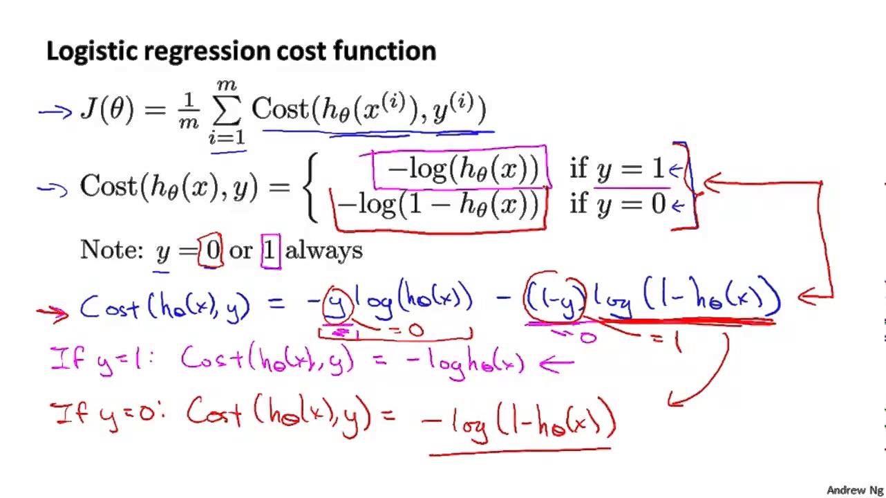
[J(\theta) = \frac{1}{m}\sum_{i = 1}^mCost(h_\theta(x^{(i)}) - y^{(i)})]
where $ Cost(h_\theta(x^{(i)}) - y^{(i)}) $ means the cost I want my learning algorithm to pay for the prediction of $ h_\theta(x^{(i)}) $ while the actual label is $ y^{(i)} $.
[Cost(h_\theta(x), y) =
\begin{cases}
-\mathrm{log}(h_\theta(x)) \space \text{if} \space y = 1
-\mathrm{log}(1 - h_\theta(x)) \space \text{if} \space y = 0
\end{cases}]
Try to plot the $ Cost(h_\theta(x), y) $ function, and get the intuition of that:
- $ Cost = 0 \space \text{if} \space y = 1, h_\theta(x) = 1 $
- $ \text{But as} \space h_\theta(x) \to 0, Cost \to \infty $
-
Captures intuition that if $h_\theta(x) = 0$ (predict $P(y = 1 x;\theta) = 0$), but $y = 1$, we’ll penalize learning algotithm by a very large cost. 
- $ Cost = 0 \space \text{if} \space y = 0, h_\theta(x) = 0 $
- $ \text{But as} \space h_\theta(x) \to 1, Cost \to \infty $
-
Captures intuition that if $h_\theta(x) = 1$ (predict $P(y = 1 x;\theta) = 1$), but $y = 0$, we’ll penalize learning algotithm by a very large cost. 
Gradient Descent
- Simplified Cost Function
[Cost(h_\theta(x), y) = -y\mathrm{log}(h_\theta(x)) - (1 - y)\mathrm{log}(1 - h_\theta(x))]
[J(\theta) = \frac{1}{m}\sum_{i=1}^mCost(h_\theta(x^{(i)}), y^{(i)})]
Minimize $ J(\theta) $ to fit parameters $ \theta $, then make a prediction given new $ x $:
[h_\theta(x) = \frac{1}{1 + e^{-\theta^Tx}}]
- Gradient Descent
Repeat until converge:
[\theta_j := \theta_j - \alpha\sum_{i=1}^m(h_\theta(x^{(i)}), y^{(i)})x_j^{(i)}]
- Vectorization
For simplicity, you may apply this trick:
If you want an (n * 1) vector, then you have to multiply an (n * m) matrix with a (m * 1) vector.
Or see the photo below:

Advanced Optimization
Given $ \theta $, we have code that can compute
- $ J(\theta) $
- $ \frac{\partial}{\partial\theta_j}J(\theta) $ (for $ j = 0, 1, \dots, n $)
Then we could use all of these optimization algorithm to minimize $ J(\theta) $:
- Gradient descent
- Conjugate gradient
- BFGS
- L-BFGS
The last three have these advantages below:
- No need to manually pick $ \alpha $
- Often faster than gradient descent.
And the disadvantage is:
- More complex
code to calculate $ J(\theta) $ and $ \frac{\partial}{\partial\theta_j}J(\theta) $ (for $ j = 0, 1, \dots, n $):
function [jVal, gradient] = costFunction(theta)
jVal = % code to compute J(theta)
gradient(1) = % code to compute partial derivative of J(theta) in terms of theta(1)
gradient(2) = % code to compute partial derivative of J(theta) in terms of theta(2)
...
gradient(n+1) = % code to compute partial derivative of J(theta) in terms of theta(n)
code to use more complex optimization algorithm:
options = optimset('GradObj', 'on', 'MaxIter', '100'); % options parameters
initialTheta = zeros(2, 1); % initial guess for theta
[optTheta, functionVal, exitFlag] = fminunc(@costFunction, initialTheta, options); % costFunction is defined by ourselves, initialTheta should be at least 2-d
One-vs-all
Train a logistic regression classifier $ h_{\theta}^{(i)}(x) $ for each class $ i $ to predict the probability that $ y = i $.
On a new input $ x $, to make a prediction, pick the class $ i $ that maximizes:
[\max\limits_{i}h_{\theta}^{(i)}(x)]
Overfitting
In linear regression:
- Having too many features, the learned hypothesis may fit the training set very well ($ J(\theta) = \frac{1}{2m}\sum_{i=1}^m(h_\theta(x^{(i)}) - y^{(i)})^2\approx0 $), but fail to generalize to new examples (predict prices on new examples).
The same thing in logistic regression.
Options:
- Reduce number of features.
- Manually select which features to keep.
- Model selection algorithm.
- Regularization.
- Keep all the features, but reduce magnitude/values of parameters $ \theta_j $.
- Works well when we have a lot of features, each of which contributes a bit to predicting $ y $,
Regularized Linear Regression
- Cost Function
Shrinking down all the parameters by adding them in cost function:(penalize all the parameters except for $ \theta_0 $)
[J(\theta) = \frac{1}{2m}[\sum_{i=1}^m(h_\theta(x^{(i)}) - y^{(i)})^2 + \lambda\sum_{j=1}^n\theta_j^2]]
where $ \lambda $ is the regularization parameter. Then we try to:
[\min\limits_{\theta}J(\theta)]
- What if $ \lambda $ is set to an extremely large value (perhaps for too large for our problem, say $ \lambda = 10^{10} $)?
- We would penalize parameters too heavy($ \theta_1\approx0, \theta_2\approx0, \theta_3\approx0, \dots $)
- Underfit.
- Gradient Descent
Repeat until converge:
- $ \theta_0 := \theta_0 - \alpha\frac{1}{m}\sum_{i=1}^m(h_\theta(x^{(i)}) - y^{(i)})x_0^{(i)} $
- $ \theta_j := \theta_j(1 - \alpha\frac{\lambda}{m}) - \alpha\frac{1}{m}\sum_{i=1}^m(h_\theta(x^{(i)}) - y^{(i)})x_j^{(i)} $
where usually $ 1 - \alpha\frac{\lambda}{m} < 1 $, and $ h_\theta(x) = \theta^Tx $.
Regularized Normal Equation
[\theta = (X^TX + \lambda
\begin{bmatrix}
0
& 1
&& 1
&&& \ddots
&&&& 1
\end{bmatrix})^{-1}X^Ty]
Regularized Logistic Regression
- Cost Function
[J(\theta) = -[\frac{1}{m}\sum_{i=1}^my^{(i)}\log h_\theta(x^{(i)}) + (1 - y^{(i)})\log(1 - h_\theta(x^{(i)}))] + \frac{\lambda}{2m}\sum_{j=i}^n\theta_j^2]
- Gradient Descent
Repeat until converge:
- $ \theta_0 := \theta_0 - \alpha\frac{1}{m}\sum_{i=1}^m(h_\theta(x^{(i)}) - y^{(i)})x_0^{(i)} $
- $ \theta_j := \theta_j(1 - \alpha\frac{\lambda}{m}) - \alpha\frac{1}{m}\sum_{i=1}^m(h_\theta(x^{(i)}) - y^{(i)})x_j^{(i)} $
where usually $ 1 - \alpha\frac{\lambda}{m} < 1 $, and $ h_\theta(x) = \frac{1}{1 + e^{-\theta^Tx}} $.(note that it is not the same as linear regression)